By Jean-Louis Queguiner
 Where does Neural come from?
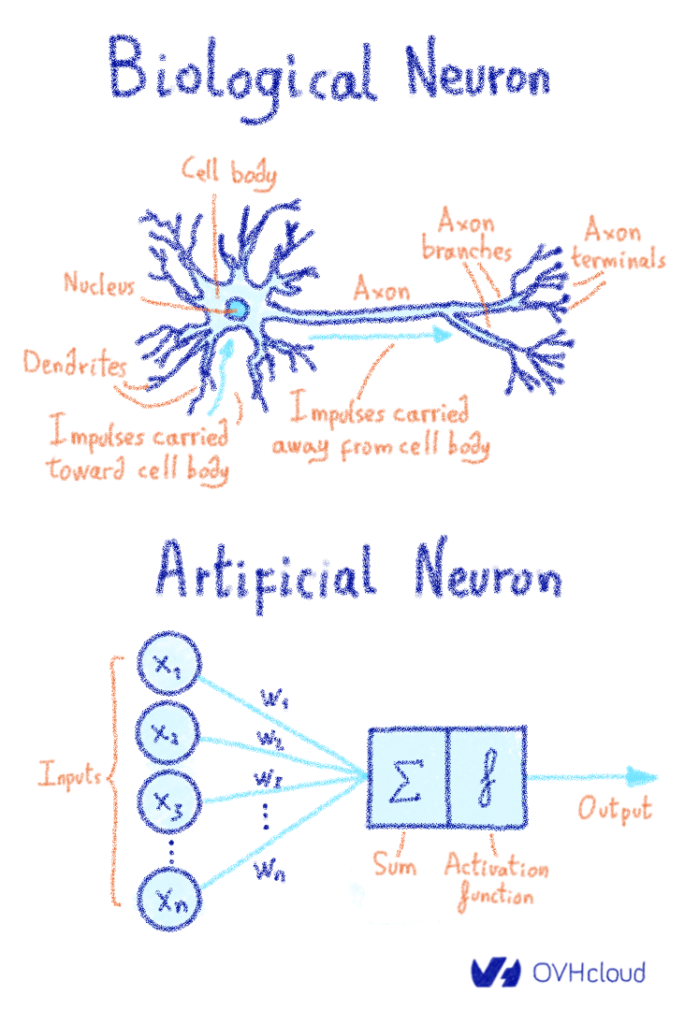
As you should know, a biological neuron is composed of multiple dendrites, a nucleus and a axon (if only you had paid attention in your biology classes). When a stimuli is sent to the brain, it is received through the synapse located at the extremity of the dendrite.
When a stimuli arrives at the brain it is transmitted to the neuron via the synaptic receptors which adjust the strength of the signal sent to the nucleus. This message is transported by the dendrites to the nucleus to then be processed in combination with other signals emanating from other receptors on the other dendrites. Thus the combination of all these signals takes place in the nucleus. After processing all these signals, the nucleus will emit an output signal through its single axon. The axon will then stream this signal to several other downstream neurons via its axon terminations. Thus a neuron analysis is pushed in the subsequent layers of neurons. When you are confronted with the complexity and efficiency of this system, you can only imagine the millennia of biological evolution that brought us here.
On the other hand, artificial neural networks are built on the principle of bio-mimicry. External stimuli (the data), whose signal strength is adjusted by the neuronal weights (remember the synapse?, circulates to the neuron (place where the mathematical calculation will happen) via the dendrites. The result of the calculation called the output is then re-transmitted (via the axon) to several other neurons and then subsequent layers are combined, and so on.
Therefore, their is a clear parallel between biological neurons and artificial neural networks as presented in the figure below.
 The Artificial Neural Network Recipe
To build a good Artificial Neural Network (ANN) you will need the following ingredients
Ingredients:Artificial Neurons (processing node) are composed of:
(many) input neuron(s) connection(s) (dendrites)
a computation unit (nucleus) composed of:
a linear function (ax+b)
an activation function (equivalent to the synapse)
An output (axon)
Preparation to get an ANN for image classification training:1. Decide on the number of output classes (meaning the number of image classes for example, two for cat vs. dog)
2. Draw as many computation units as the number of output classes (congrats you just created the Output Layer of the ANN)
3. Add as many Hidden Layers as needed within the defined architecture (for instance vgg16 or any other popular architecture). Tip Hidden Layers are just a set of neighboured Compute Units, they are not linked together.
4. Stack those Hidden Layers to the Output Layer using Neural Connections
5. It is important to understand that the Input Layer is basically a layer of data ingestion
6. Add an Input Layer that is adapted to ingest your data (or you will adapt your data format to the pre-defined architecture)
7. Assemble many Artificial Neurons together in a way where the output (axon) a Neuron on a given Layer is (one) of the input of another Neuron on a subsequent Layer. As a consequence, the Input Layer is linked to the Hidden Layers which are then linked to the Output Layer (as shown in the picture below) using Neural Connections (also shown in the picture below).
8. Enjoy your meal
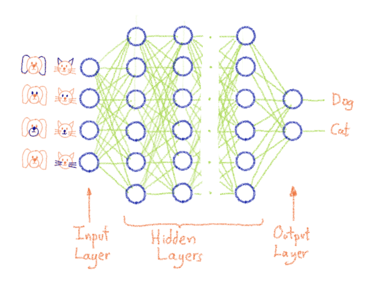
simplified schema of a neural network architecture
What does it mean to train an Artificial Neural Network?All Neurons of a given Layer are generating an Output, but they dont have the same Weight for the next Neurons Layer. This means that if a Neuron on a layer observes a given pattern it might mean less for the overall picture and will be partially or completely muted. This is what we call Weighting: a big weight means that the Input is important and of course a small weight means that we should ignore it. Every Neural Connection between Neurons will have an associated Weight.
And this is the magic of Neural Network Adaptability: Weights will be adjusted over the training to fit the objectives we have set (recognize that a dog is a dog and that a cat is a cat). In simple terms: Training a Neural Network means finding the appropriate Weights of the Neural Connections thanks to a feedback loop called Gradient Backward propagation
and thats it folks.
Parallel between Control Theory and Deep Learning TrainingThe engineering field of control theory defines similar principles to the mechanism used for training neural networks.
Control Theory general conceptsIn control systems, a setpoint is the target value for the system.
A setpoint (input) is defined and then processed by a controller, which adjusts the setpoints value according to the feedback loop (Manipulated Variable). Once the setpoint has been adjusted it is then sent to the controlled system which will produce an output. This output is monitored using an appropriate metric which is then compared (comparator) to the original input via a feedback loop. This allows the controller to define the level of adjustment (Manipulated Variable) of the original setpoint.
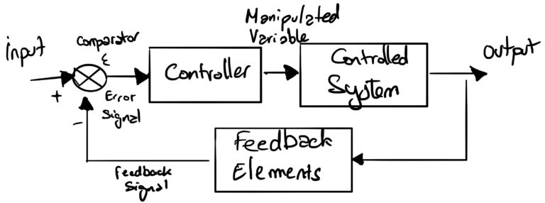 Control Theory applied to a radiator
Lets take the example of a resistance (controlled system) in a radiator. Imagine you decide to set the room temperature to 20 ° C (setpoint). The radiator starts up, supplies the resistance with a certain intensity defined by the controller. A probe (thermometer) will then take the ambient temperature (feedback elements) which is then compared (comparator) to the setpoint (desired temperature) and adjusts (controller) the electric intensity sent to the resistance. The adjustment of the new intensity is deployed via an incremental adjustment step.
Control Theory applied to Neural Network TrainingThe training of a neuron network is similar to a radiator insofar as the controlled system is the cat or dog detection model.
The objective is no longer to have the minimum difference between the setpoint temperature and the actual temperature but to minimize the error (Loss) between the classification of the incoming data (a cat is a cat) and the one made by the neural network.
In order to achieve this, the system will have to look at the input (setpoint) and compute an output (controlled system) based on the parameters defined in the algorithm. This phase is called the forward pass.
Once the output has been calculated, the system will re-propagate the evaluation error using Gradient Retro-propagation (Feedback Elements). While the temperature difference between the setpoint and the thermometer was converted into electrical intensity for the radiator, here the system will adjust the weights of the different inputs into each neuron with a given step (learning rate).
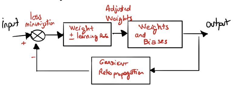 Parallel between electrical engineering controlled system and neural network training processOne thing to consider: The Valley Problem
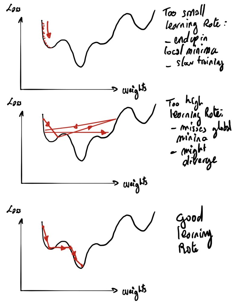
When training the system, the backward propagation will lead the system to reduce the error its making to best fit the objectives you have set (finding that a dog is a dog
).
Choosing the learning rate at which you will adjust your weights (what one call adjustment step in Control Theory).
Just as is the case in control theory, the control system can face several issues if it is not designed correctly:
1. If the correction step (learning rate) is too small it will lead to a very slow convergence (i.e. it will take a very long time to get your room to 20°C
).
2. Too small a learning rate can also lead to you being stuck in a local minim
3. If the correction step (learning rate) is too high it will lead the system to never converge (beat around the bush) or worse (i.e. the radiator will oscillate between being either too hot or too cold)
4. The system could enter into a resonance state (divergence).
 In the end Training an Artificial Neural Network (ANN) requires just a few steps:
1. First an ANN will require a random weight initialization
2. Split the dataset in batches (batch size)
3. Send the batches 1 by 1 to the GPU
4. Calculate the forward pass (what would be the output with the current weights)
5. Compare the calculated output to the expected output (loss)
6. Adjust the weights (using the learning rate increment or decrement) according to the backward pass (backward gradient propagation).
7. Go back to square 2
Further noticeThats all folks, you are now all set to read our future blog post which focuses on Distributed Training in a Deep Learning Context.
Source: OVHcloud Blog
Original Content:
https://shorturl.at/GZ047