Shanthababu Pandian Introduction
Data Engineers and Data Scientists need data for their Day-to-Day job. Of course, It could be for Data Analytics, Data Prediction, Data Mining, Building Machine Learning Models Etc., All these are taken care of by the respective team members and they need to work towards identifying relevant data sources, and associated with the business problems.
Data SourcesData Sources can be identified in two different ways.
Functional aspects
Technical aspects
1 Functional aspectWith respect to functional aspects, it can be sub-divided into Primary and Secondary sources. Lets quickly discuss this.
Primary Sources: Data in the form of documents, a person details (First Name/Last Name/Address/Date of Birth/Phone Number/Passport Number/Drivers License/Aadar card/SSN/National ID Number and etc.,)
Secondary Sources: Derived from Primary.
2 Technical aspectsBoth above said is nothing but in the form of non-digital form. When we convert them into meaningful ways. then it got the feel of technical rhythm. Then it would be given the way to below divisions
Relational ( Relational Data Model)
Multidimensional (OLAP Data Model)
 What is Data Handling?
It refers to the set of processes, Lets will walk through them one by one in detail along with effective python libraries
Data-collection
Data cleaning/cleansing
Data preparation
Data Wrangling
Data-Collection (DC)General statements about DATA COLLECTION is a highly time-consuming and manual intervention, but in this digital world, it would be from an application source, mobile application, IoT devices etc., using automated tools and technologies.
Conducting a campaign
Quantitative research
Interviews
Observation and research
Online Sales/Marketing analysis
Social Media
IoT and IIOT
Collecting data from Clients/Customers/End-users is a key process and business strategy to reach your perfect target audience to improve your presence in the leading market and support. So, in recent years industries are funding to collect data and draft big game plans for their business advancements.
Source
https://www.fotolog.com/steps-in-data-science-process/Why is so important?From the data collection,
We could analyze the root level information and identify your existing and potential customers in the market.
You can build customer relationships strong and plan for your future marketing space
Data in digital format would remove potential bias
Data-Collection is the first and major step in the Machine Learning(ML) life cycle. specifically for training, testing and building the right ML model to address the problem statement. The data which were collecting will define the outcome of the ML systems after lots of iterations and the process, So this process is very important for Data Science (or) ML team. Obviously, there are multiple challenges during this period, lets review a few of them here.
The collected data should be related to the problem statement.
Inaccurate, missing data, null values in columns, and irrelative/missing images from the source would lead to errored prediction.
Imbalance, an anomaly, and outliers are deviating from our focus and take us to the under-represented stage of model building.
Strategies to fix the challenges and issues with DC
Pre-cleaned, freely available datasets. If the problem statement aligns with a cleaned, properly drafted dataset, then take advantage of existing, open-source expertise.
Web crawling and scraping methods to collect the data using bots and automated tools.
Private data. ML engineers can create their own data when the volume of data is required to train the model is very small and does not align with the problem statement.
Custom data, Organizations can create the data.
Data cleaning/cleansingIn the ML lifecycle, 60% or more of that timeline will be demanded in Data Preparation, Loading, Cleaning/Cleansing, Transforming and reshaping/rearranging.
When we start looking at the Cleaning (or) Cleansing process, The below list of options is provided by Python.
Missing Data handling techniques
Transformation of Data
Manipulation Methods
Missing Data handling techniques: Missing data analysis is a very common technique in the ML world. Data missing impacts the analysis and model. Certainly, the model couldnt train properly and misguide the prediction or forecasting at a later point.
In Pythons pandas, we use to adapt NA (Not Available or Not exist)
(i) Finding Null values
I will show a few sample codes here
(a) Output if Null item in the list, it should be NaN
import pandas as pd
import numpy as np
string_collection=pd.Series(['Apple','Ball','Cat',np.nan,'Dog'])
string_collection
0 Apple
1 Ball
2 Cat
3 NaN
4 Dog
dtype: object
(b) Output if Null item in the list, it should be True
string_collection.isnull()
0 False
1 False
2 False
3 True
4 False
dtype: bool
(c) Dropping NaN from the list
string_collection.dropna()
0 Apple
1 Ball
2 Cat
4 Dog
dtype: object
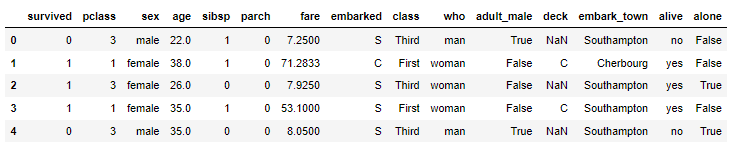
(d) Lets try with the titanic dataset
import numpy as np
import pandas as pd
import matplotlib.pyplot as plt
import seaborn as sns
%matplotlib inline
df_titanic = pd.read_csv(titanic.csv)
df_titanic.head()
df_titanic.isnull().any()
(d) Number of Null in the column(s)
print("Number of Null in age column:",df_titanic['age'].isnull().sum())
print("Number of Null in embark_town column:",df_titanic['embark_town'].isnull().sum())
Number of Null in age column: 177
Number of Null in embark_town column: 2
(e) Null values through heatmap
sns.heatmap(df_titanic.isnull(),yticklabels=False,cbar=False,cmap='viridis')
(ii) Filtering the missing data: There are two ways to filter out the missing values either by using dropna or notnull.
dropna will remove the row from the dataset/series
notnull still data will be in the dataset/series
NaN handling methods in pandas
Methods Notes
isnull returns boolean for specified column/variable
notnull excluding the null values/rows
fillna filling with the specified value
dropna dropping row(s)
Usage
(a)Filtering Using Notnull/ Dropna rows
import pandas as pd
import numpy as np
from numpy import nan as NA
data=pd.Series([100,250,NA,350,400,500,NA,950])
print(data)
print("Apply dropna")
print("=============")
print(data.dropna() )
print("Apply notnull")
print("=============")
print(data[data.notnull()])
Output
0 100.0
1 250.0
2 NaN
3 350.0
4 400.0
5 500.0
6 NaN
7 950.0
dtype: float64
Apply dropna
=============
0 100.0
1 250.0
3 350.0
4 400.0
5 500.0
7 950.0
dtype: float64
Apply notnull
=============
0 100.0
1 250.0
3 350.0
4 400.0
5 500.0
7 950.0
dtype: float64
(iii) Filtering the NA from dataframe
import pandas as pd
import numpy as np
from numpy import nan as NA
data=pd.DataFrame([[100,101,102],['Raj','John',NA],[NA,NA,NA],['Chennai','Bangalore','Delhi']])
print(data)
Output
0 1 2
0 100 101 102
1 Raj John NaN
2 NaN NaN NaN
3 Chennai Bangalore Delhi
(iv) Cleaning NA
Cleand_data=data.dropna()
print(Cleand_data)
Output
0 1 2
0 100 101 102
3 Chennai Bangalore Delhi
So far we have discussed filtering the missing data, but cleaning is not only the solution. in a real-time scenario, we can not remove just like that without the opinion from Subject Matter Experts (SMEs). Need to fill in the data. there are various techniques are there. Lets will discuss, a few of them in this article.
import pandas as pd
import numpy as np
from numpy import nan as NA
data=pd.DataFrame([[100,101,102],['Raj','John','Jay'],[NA,NA,NA],['Chennai','Bangalore','Delhi']])
data.fillna(0)
Output
0 1 2
0 100 101 102
1 Raj John Jay
2 0 0 0
3 Chennai Bangalore Delhi
(v) Fill in the data from the previous row
import pandas as pd
import numpy as np
from numpy import nan as NA
data=pd.DataFrame([['Raj','John','Jay'],[100,101,102],[NA,NA,NA],['Chennai','Bangalore','Delhi']])
print(data)
Output
0 1 2
0 Raj John Jay
1 100 101 102
2 NaN NaN NaN
3 Chennai Bangalore Delhi
data.fillna(method='ffill')
0 Raj John Jay
1 100 101 102
2 100 101 102
3 Chennai Bangalore Delhi
Will see this from a dataframe point of view.
(vi) Removing Duplicates rows from the dataframe, just using drop_duplicates
import pandas as pd
import numpy as np
from numpy import nan as NA
data=pd.DataFrame([['Raj','Chennai'],['John','Chennai'],['Jey','Bangalore'],['Mohan','Delhi'],['Raj','Channai']])
print(data)
Output
0 1
0 Raj Chennai
1 John Chennai
2 Jey Bangalore
3 Mohan Delhi
4 Raj Channai
(vii) Finding duplicates
data.duplicated()
0 False
1 False
2 False
3 False
4 True
dtype: bool
data.drop_duplicates()
0 1
0 Raj Chennai
1 John Chennai
2 Jey Bangalore
3 Mohan Delhi
(viii) Replacing Values
import pandas as pd
import numpy as np
from numpy import nan as NA
data=pd.DataFrame([['Raj','Chennai',0],['John','Chennai',2],['Jey','Bangalore',-1],['Mohan','Delhi',-3]])
print(data)
Output
0 Raj Chennai 0
1 John Chennai 2
2 Jey Bangalore 0
3 Mohan Delhi 0
With mean() in a dataset, Consider that the given auto-mpg has null values in the horsepower column, and some junk data (like ? ).
print(df_cars["horsepower"].isna().sum())
Output
19
So, the horsepower column has 19 null values, lets handle this now.
df_cars.horsepower = df_cars.horsepower.str.replace('?','NaN').astype(float)
df_cars.horsepower.fillna(df_cars.horsepower.mean(),inplace=True)
df_cars.horsepower = df_cars.horsepower.astype(int)
print("######################################################################")
print(" After Cleaning and type convertion in the Data Set")
print("######################################################################")
df_cars.info()
Null values are replaced by mean of the horsepower column.
print(df_cars["horsepower"].isna().sum())
Output
0
Yes! We did it! awsome. Now we could consider the horsepower column is clean and error-free.
Data Transforming(I) Filtering Outliers: In simple terms, we can analyze the data distribution identify the outliers, and remove them from the dataset to avoid overfitting or underfitting during model evaluation. Mathematically finding the outliers really challenging process, surely will use visualization techniques will support ease and understanding better.
import pandas as pd
import numpy as np
import matplotlib.pyplot as plt
import seaborn as sns
import pandas as pd
import numpy as np
import matplotlib.pyplot as plt
import seaborn as sns
from IPython.display import display
import statsmodels as sm
from scipy import stats
df_cars = pd.read_csv("auto-mpg.csv")
df_cars.horsepower = df_cars.horsepower.str.replace('?','NaN').astype(float)
df_cars.horsepower.fillna(df_cars.horsepower.mean(),inplace=True)
df_cars.horsepower = df_cars.horsepower.astype(int)
sns.boxplot(x=df_cars["horsepower"])
Image Source: Author
We could observe that there is an outlier (dots)
after the scale of 200 for the horsepower feature. Lets remove the outliers
using mathematical ways.
z_scores = stats.zscore(df_cars["horsepower"])
abs_z_scores = np.abs(z_scores)
print(abs_z_scores)
Output
[0.67155703 1.5895576 1.19612879 1.19612879 0.93384291 2.455101
3.03212994 2.900987 3.16327288 2.2452723 1.72070054 1.45841466
1.19612879 3.16327288 0.24644355 0.24644355 0.19398637 0.50872943
0.43004366 1.53164436 0.45627225 0.37758649 0.24644355 0.22567103
0.37758649 2.900987 2.50755818 2.76984406 2.32395806 0.43004366
0.37758649 0.24644355 0.01038626 0.11530061 0.01584233 0.11530061
0.43004366 0.11530061 1.5895576 1.85184348 1.27481455 1.19612879
1.98298642 1.72070054 1.85184348 0.14698527 0.84970107 0.11530061
0.43004366 0.48250084 0.37758649 0.90215825 0.74478672 1.03330119
0.92838683 1.16444413 0.90215825 0.24644355 0.63987237 1.32181565
0.37758649 0.48250084 1.5895576 1.85184348 1.19612879 1.27481455
1.19612879 2.71738688 1.32727172 1.45841466 2.2452723 0.19398637
1.19612879 0.67155703 0.93384291 1.19612879 0.19944245 0.74478672
0.45627225 0.92838683 0.48250084 0.32512931 0.19398637 0.63987237
0.43004366 1.85184348 1.19612879 1.06498585 0.85515714 1.19612879
2.455101 1.19612879 1.40595749 1.19612879 2.900987 3.16327288
1.85184348 0.01584233 0.11530061 0.11530061 0.43004366 0.24644355
1.53164436 1.19612879 1.64201478 1.72070054 1.98298642 0.11530061
0.43004366 0.84970107 0.27267214 0.37758649 0.50872943 0.06829951
0.37758649 1.06498585 3.29441582 1.45295859 0.77101531 0.3513579
0.19944245 1.19612879 0.14698527 0.46172832 1.98298642 0.24644355
0.01038626 0.11530061 0.11530061 0.98084401 0.63987237 1.03330119
0.77101531 0.11530061 0.14698527 0.01584233 0.93384291 1.19612879
1.19612879 0.93384291 1.19612879 0.5611866 0.98084401 0.69232954
1.37427283 1.13821554 0.77101531 0.77101531 0.77101531 0.19398637
0.29890072 0.98084401 0.24644355 0.01584233 0.84970107 0.84970107
1.72070054 1.06498585 1.19612879 1.14367161 0.14698527 0.01584233
0.14698527 0.24644355 0.14698527 0.14698527 0.64532844 0.77101531
0.5611866 0.11530061 0.69232954 0.22021496 0.87592966 0.19398637
0.19398637 0.90215825 0.37758649 0.24644355 0.43004366 0.16775779
0.27812821 1.34804424 0.48250084 0.61364378 0.32512931 0.66610096
0.5611866 0.93384291 1.19612879 0.40927115 1.24858596 0.11530061
0.01584233 0.61364378 0.37758649 1.37427283 1.16444413 0.90215825
1.34804424 0.11530061 0.69232954 0.14698527 0.24644355 0.87592966
0.90215825 0.77101531 0.84970107 0.06284343 1.19612879 0.43004366
0.09452809 0.40927115 1.98298642 1.06498585 0.67155703 1.19612879
0.95461542 0.63987237 1.2169013 0.22021496 0.90215825 1.06498585
0.14698527 1.06498585 0.67155703 0.14698527 0.01584233 0.11530061
0.16775779 1.98298642 1.72070054 2.2452723 1.1699002 0.69232954
0.43004366 0.77101531 0.40381508 1.08575836 0.5611866 0.98084401
0.69232954 0.19398637 0.14698527 0.14698527 1.47918718 1.0070726
1.37427283 0.90215825 1.16444413 0.14698527 0.93384291 0.90761432
0.01584233 0.24644355 0.50872943 0.43004366 0.11530061 0.37758649
0.01584233 0.50872943 0.14698527 0.40927115 1.06498585 1.5895576
0.90761432 0.93384291 0.95461542 0.24644355 0.19398637 0.77101531
0.24644355 0.01584233 0.50872943 0.19398637 0.03661485 0.54041409
0.27812821 0.75024279 0.87592966 0.95461542 0.27812821 0.50872943
0.43004366 0.37758649 0.14698527 0.67155703 0.64532844 0.88138573
0.80269997 1.32727172 0.98630008 0.54041409 1.19612879 0.87592966
1.03330119 0.63987237 0.63987237 0.71855813 0.54041409 0.87592966
0.37758649 0.90215825 0.90215825 1.03330119 0.92838683 0.37758649
0.27812821 0.27812821 0.37758649 0.74478672 1.16444413 0.90215825
1.03330119 0.37758649 0.43004366 0.37758649 0.37758649 0.69232954
0.37758649 0.77101531 0.32512931 0.77101531 1.03330119 0.01584233
1.03330119 1.47918718 1.47918718 0.98084401 0.98084401 0.98084401
0.01038626 0.98084401 1.11198695 0.7240142 0.11530061 0.43004366
0.01038626 0.84970107 0.53495802 0.53495802 0.32512931 0.14698527
0.53495802 1.2169013 1.05952977 1.16444413 0.98084401 1.03330119
1.11198695 0.95461542 1.08575836 1.03330119 1.03330119 0.79724389
0.01038626 0.77101531 0.77101531 0.11530061 0.79724389 0.63987237
0.74478672 0.3043568 0.40927115 0.14698527 0.01584233 0.43004366
0.50872943 0.43004366 0.43004366 0.43004366 0.50872943 0.53495802
0.37758649 0.32512931 0.01038626 0.79724389 0.95461542 0.95461542
1.08575836 0.90215825 0.43004366 0.77101531 0.90215825 0.98084401
0.98084401 0.98084401 0.14698527 0.50872943 0.32512931 0.19944245
0.22021496 0.53495802 0.37758649 0.48250084 1.37427283 0.53495802
0.66610096 0.58741519 0.69232954]
I can understand that this is really all, thats fine lets set up a threshold and continue.
filtered_entries = (abs_z_scores < 1.5)
new_df = df_cars[filtered_entries]
print(new_df)
mpg cylinders displacement horsepower weight acceleration
0 18.0 8 307.0 130 3504 12.0
2 18.0 8 318.0 150 3436 11.0
3 16.0 8 304.0 150 3433 12.0
4 17.0 8 302.0 140 3449 10.5
11 14.0 8 340.0 160 3609 8.0
.. ... ... ... ... ... ...
394 44.0 4 97.0 52 2130 24.6
395 32.0 4 135.0 84 2295 11.6
396 28.0 4 120.0 79 2625 18.6
397 31.0 4 119.0 82 2720 19.4
398 NaN 4 250.0 78 2500 18.5
model_year origin name
0 70.0 1.0 chevrolet chevelle malibu
2 70.0 1.0 plymouth satellite
3 70.0 1.0 amc rebel sst
4 70.0 1.0 ford torino
11 70.0 1.0 plymouth 'cuda 340
.. ... ... ...
394 82.0 2.0 vw pickup
395 82.0 1.0 dodge rampage
396 82.0 1.0 ford ranger
397 82.0 1.0 chevy s-10
398 NaN NaN NaN
[360 rows x 9 columns]
sns.boxplot(x=new_df["horsepower"])
Image Source: Author
Now, the box plot is very clear and has no more
outliers. Think about the power of python libraries here.
(II) Converting Type: We Will analyze the given dataset columns type, this is an essential activity before we do feature engineering and test training.
df_cars = pd.read_csv("auto-mpg.csv")
print("############################################")
print(" Info Of the Data Set")
print("############################################")
df_cars.info()
Output
Image Source: Author
Observation:
1. we could observe that the features and its data type, along with count Null
2. horsepower and name features are, Object in the given data set
How to transform this into a meaningful way for our analysis. using simple astype.
df_cars.horsepower = df_cars.horsepower.str.replace('?','NaN').astype(float)
df_cars.horsepower.fillna(df_cars.horsepower.mean(),inplace=True)
df_cars.horsepower = df_cars.horsepower.astype(int)
print("######################################################################")
print(" After Cleaning and type convertion in the Data Set")
print("######################################################################")
df_cars.info()
Output
Observation:
1. we could observe that the features and its data type, along with count Null
2. we could observe that horsepower is now int type.
(III) Create Dummy Variables: In a real-time scenario, wehave to handle the categorical variable in intelligent ways so that we could accommodate them in the process of converting them into dummy variables and make use of them as independent variables. Lets see the sample here.
df_cars.head(5)
Image Source: Author
Lets convert them into a Categorical variable
df_cars['origin'] = df_cars['origin'].replace({1: 'america', 2: 'europe', 3: 'asia'})
df_cars.head()
Image Source: Author
cData = pd.get_dummies(df_cars, columns=['origin'])
cData
Image Source: Author
(III) String Transforming: In some situations, we have to deal with string values in the given dataset and as data scientists, we are responsible for streamlining them for data analysis. Here is one classical sample most commonly facing.
pattern = chevroelt|chevy|chevrolet
mask = df_cars[name].str.contains(pattern, case=False, na=False)
df_cars[mask].head()
Image Source: Author
Observe here that Chevrolet in different spellings, So during classification modeling this would give you headache and challenging your patience, Now follow me, how we can handle this.
# Correct name
df_cars['name'] = df_cars['name'].str.replace('chevroelt|chevrolet|chevy','chevrolet')
df_cars['name'] = df_cars['name'].str.replace('maxda|mazda','mazda')
df_cars['name'] = df_cars['name'].str.replace('mercedes|mercedes-benz|mercedes benz','mercedes')
df_cars['name'] = df_cars['name'].str.replace('toyota|toyouta','toyota')
df_cars['name'] = df_cars['name'].str.replace('vokswagen|volkswagen|vw','volkswagen')
The above code will streamline the brand names and your modeling will give perform better than earlier.
Lets see how to string transformation works here.
pattern = 'chevrolet'
mask = df_cars['name'].str.contains(pattern, case=False, na=False)
df_cars[mask].head()
Hope you love this, Yes! I can understand.Read more articles on our website about data handling techniques. Click here.
ConclusionThis is a long journey, so far we covered the possible and most frequent techniques in Data Handling techniques right from data collection, cleaning, and wrangling aspects, still, many more techniques are there and usage is dependent on the cases, With respect to Data Science, the data handling is a vital role and 60-65% of effort would require to fine-tune our data for modeling, So remember all these features we had discussed over here certainly help you a lot, Let me say break and will connect with you all on something interesting topics. Hope you liked my article on data handling techniques.
Thanks for your time, Good Luck! See you all soon. Shanthababu
Source: TechTarget, Inc
Original Content:
https://shorturl.at/ACFR8


